All you need is R Markdown!

Introduction

There exist a wide variety of options to write research papers, presentations, and technical reports. Among them, the most typical ones in my experience include MS Office, LaTeX/Beamer, GoogleDocs, Dropbox Papers, among others. These documents share the same disadvantage when working with data: they don’t have the capabilities to execute statistical analysis codes within the manuscript.

When you work mainly with data analysis, as I do, the separation between the codes in where you perform the statistical analysis and the document produces several problems that must be faced. In the first place, this separation increases the risk of typing errors. When you are copying and pasting coefficients, numbers, or tables, there is always a probability in which you make a mistake that you will not notice later. In the second place, this separation increases the amount of work that you have to spent when updating tables and figures. These non-static attributes continuously change as we modify samples and models, and sincerely, copying and pasting images, again and again, is not a funny or efficient practice. Finally, when the code is not in the document, reproducibility became a more challenging task for a third party interested in your research.

Because I have encountered all the problems that I mentioned above, I started to work in R Markdown. This tool is an enriched Markdown document, configured with a YAML header, that allows you to execute code (R, python, JS, among others) together with text (including LaTeX syntax) within the same notebook and produce outputs in various formats, including HTML and PDF.

I want to share some helpful practices that I adopted using R Markdown notebooks for all the online community in this post. Since R Markdown has many capabilities apart from manuscripts (i.e., Slides and Dashboards), I will focus on documents, especially in PDF outputs. It is worth mentioning that this post is not a complete revision of this fantastic tool’s capabilities. Here, I tried to share my experience and include most of the tricks I use while working on my documents. Hope this post will help you!

(The original .Rmd file used for this post is here. It is not exactly the same because the .md output it is not full compatible with the site’s theme!)

Creating an `R Markdown` document

My preferred IDE to work in R Markdown is RStudio. To create a new notebook in RStudio, just click File > New File > R Markdown. You can specify the document type, output type (HTML, PDF, Word), and the template for each document type.

Markdown

In my opinion, one of the features that make R Markdown an easy-to-learn language is Markdown syntax. “Markdown is a text-to-HTML conversion tool for web writers. Markdown allows you to write using an easy-to-read, easy-to-write plain text format, then convert it to structurally valid XHTML (or HTML). (John Gruber)”. This language is super easy to learn, and it is simple to format. For instance:

## Header

*Italic Letters*

**Bold Letters**

* List
* List
* List

1. Numbered List
2. Numbered List
3. Numbered List

`code`

Hello, I'm writing some text in my `R Markdown` document. Markdown is super easy to use!

[Check more tips and tricks](https://www.markdownguide.org/cheat-sheet/)

Italic Letters

Bold Letters

List
List
List

Numbered List
Numbered List
Numbered List

code

Hello, I’m writing in my R Markdown document. Markdown is super easy to use!

Check more tips and tricks

Executing code within an `R Markdown` Document.

Run code in R Markdown is straightforward. You only need to create a chunk of code using "``”`. Alternatively, if you use RStudio (which is the IDE that I definitely recommend for coding in R), you can use the option “Insert a new code chunk.”

{r My example Chunk that is not going to be executed, eval=FALSE}
print('Hello World')

I usually run a Setup chunk at the beginning of all my R Markdown documents. In all my projects, I include a settings.R script where I load all the packages thet I will use together with the local paths of the users’ machines that will collaborate.

{r Setup, eval=FALSE}
knitr::opts_chunk$set(
  echo = FALSE,
  warning = F,
  error = F,
  tidy = T,
  tidy.opts = list(width.cutoff = 50),
  collapse = T,
  warning = FALSE,
  error = FALSE,
  message = FALSE,
  comment = "",
  fig.cap = " "
)
# These options are tuned for manuscript/presentation.
# They basically run R in the background except for spitting out figures/tables

# source('settings.R', echo = FALSE)

These chunks support the execution of a wide variety of codes. You can execute Python (using reticulate), JavaScript, Bash, SQL queries, and also Stata (check this post to see how).

Executing Inline Code

To execute inline code, you have to use the following: (r) yourcode without the parenthesis in the r. Let’s see a simple example using the iris dataset.

{r Loading Data}
library(datasets)
data(iris)

mean_Sepal.Lenght <- mean(iris$Sepal.Length)

For example, using the chunk above, I can introduce the mean length of Sepal in my text, which is `r mean_Sepal.Lenght`. Alternatively, I could calculate the same value (`r mean(iris$Sepal.Length)`) using the function in the inline code directly. Also, If I don't like the number of decimals, I can use `round` function to convert `r mean_Sepal.Lenght` into `r round(mean_Sepal.Lenght,2)`.

For example, using the chunk above, I can introduce the mean length of Sepal in my text, which is 5.8433333. Alternatively, I could calculate the same value (5.8433333) using the function in the inline code directly. Also, If I don’t like the number of decimals, I can use round function to convert 5.8433333 into 5.84.

Tables

My favorite way of producing tables in R Markdown is with stargazer. This package supports a wide variety of functionalities, mainly oriented for regressions tables. Check this post in which I explain how to use it and show some examples. Here, I will show two examples of how to combine stargazer with R Markdown.

In the first place, let’s produce a descriptive statistic table. We will use iris data:

{r Des Sta, results='asis', warning=FALSE, message=FALSE}
means_array <-
  c(
    mean(iris$Sepal.Length),
    mean(iris$Sepal.Width),
    mean(iris$Petal.Length),
    mean(iris$Petal.Width)
  )
sd_array <-
  c(
    sd(iris$Sepal.Length),
    sd(iris$Sepal.Width),
    sd(iris$Petal.Length),
    sd(iris$Petal.Width)
  )   
p25_array <-
  c(
    quantile(iris$Sepal.Length, 0.25),
    quantile(iris$Sepal.Width, 0.25),
    quantile(iris$Petal.Length, 0.25),
    quantile(iris$Petal.Width, 0.25)
  )   
p75_array <-
  c(
    quantile(iris$Sepal.Length, 0.75),
    quantile(iris$Sepal.Width, 0.75),
    quantile(iris$Petal.Length, 0.75),
    quantile(iris$Petal.Width, 0.75)
  )

cols <- c('Mean', 'SD', 'P25', 'P75')
rows <-
  c('Sepal.Length', 'Sepal.Width', 'Petal.Length', 'Petal.Width')

data_matrix <-
  matrix(
    data = c(means_array, sd_array, p25_array, p75_array),
    nrow = 4,
    ncol = 4,
    dimnames = list(rows, cols)
  )

library(stargazer)
stargazer(data_matrix, type = 'html', title = 'Summary Statistics Iris Data')

**Summary Statistics Iris Data**

	Mean	SD	P25	P75

Sepal.Length	5.843	0.828	5.100	6.400
Sepal.Width	3.057	0.436	2.800	3.300
Petal.Length	3.758	1.765	1.600	5.100
Petal.Width	1.199	0.762	0.300	1.800

If you are working with .html files and want to modify table attributes (width, styles, etc.), I recommend using a custom .css to achieve this. You could declare it inside the document or in an external file. You don’t need to be an expert to program these settings, just google it and change the attributes until you are Ok with the results. If you want to go further and customize your entire .html document, check this link. For instance, we are using the following css:

table, td, th {
  border: none;
  padding-left: 1em;
  padding-right: 1em;
  margin-left: auto;
  margin-right: auto;
  margin-top: 1em;
  margin-bottom: 1em;
}

My second example is for LaTeX users. I don’t like how stargazer package handles the notes below the tables and does not support an option to resize the table. In this example, I will show an application of how I solved this.

Let’s estimate a model and produce a stargazer output. An important consideration here is that we only want the code within the tabular environment. To get this, we need to specify the options header and float to FALSE. Also, as we don’t want the notes so, we will leave them empty.

{r stargazer 2, warning=FALSE, message=FALSE}
# 1) Estimate a linear model
model <- lm(Sepal.Length ~ Sepal.Width + Petal.Length + Petal.Width, data=iris)

# 2) Capture the stargazer output in an object.
out <-
  capture.output(
    stargazer(
      model,
      type = "latex",
      float = FALSE,
      header = FALSE,
      notes.label = '',
      notes = '',
      notes.append = FALSE,
      notes.align = 'l'
    )
  )

# 3) Collapse the array in a string
tex_table <- paste(out, collapse = "\n")

# 4) Define the settings of my table (title, labels, notes)
caption <- 'My title'
label <- 'tab:my_table'
notes <- 'Own elaboration based on iris data.'

After we capture the output of stargazer in an object and collapse it in a string, we can use these objects together with inline code execution to fill a custom .tex table within our document. The LaTeX table will look like this:

{=latex}
\begin{table}[H]
\centering
\caption{`(r) caption`}
\label{`(r) label`}
\resizebox{\textwidth}{!}{
`(r) tex_table`
}
\begin{minipage}{\textwidth}
\tiny \textbf{Notes}: `(r) notes` \par
\end{minipage}
\end{table}

{=latex}
\begin{table}[H]
\centering
\caption{My title}
\label{tab:my_table}
\resizebox{\textwidth}{!}{

\begin{tabular}{@{\extracolsep{5pt}}lc} 
\\[-1.8ex]\hline 
\hline \\[-1.8ex] 
 & \multicolumn{1}{c}{\textit{Dependent variable:}} \\ 
\cline{2-2} 
\\[-1.8ex] & Sepal.Length \\ 
\hline \\[-1.8ex] 
 Sepal.Width & 0.651$^{***}$ \\ 
  & (0.067) \\ 
  & \\ 
 Petal.Length & 0.709$^{***}$ \\ 
  & (0.057) \\ 
  & \\ 
 Petal.Width & $-$0.556$^{***}$ \\ 
  & (0.128) \\ 
  & \\ 
 Constant & 1.856$^{***}$ \\ 
  & (0.251) \\ 
  & \\ 
\hline \\[-1.8ex] 
Observations & 150 \\ 
R$^{2}$ & 0.859 \\ 
Adjusted R$^{2}$ & 0.856 \\ 
Residual Std. Error & 0.315 (df = 146) \\ 
F Statistic & 295.539$^{***}$ (df = 3; 146) \\ 
\hline 
\hline \\[-1.8ex] 
\multicolumn{2}{l}{} \\ 
\end{tabular} 
}
\begin{minipage}{\textwidth}
\tiny \textbf{Notes}: Own elaboration based on iris data. \par
\end{minipage}
\end{table}

I want to highlight some essential features. In the first place, you must declare {=latex} in the chunk’s header. This will allow R Markdown and the LaTeX compiler to know that all the code within that chunk must be interpreted as LaTex code. This will save you a lot of problems while compiling the document to pdf. In the second place, remember that it is necessary to include the package float in your header if you want to specify the option [H] in the table environment. I will cover this topic later!

Figures

To include a figure, just create it using plot or ggplot.

{r FigureExample, fig.cap="Quadratic Function"}
x <- 1:100
y <- (1:100)^2

plot(x, y)

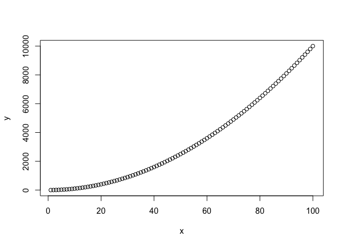
(\#fig:FigureExample)Quadratic Function

To include a figure, just create it using plot or ggplot. If you don’t want the code chunk to appear in the document, specify the option echo=FALSE in the chunk’s header. Also, some functions will print some warnings and messages. If you want to turn them off, also include warning=FALSE, message=FALSE in the header. This functionality applies to all the chunks, not only the ones that have figures.

{r Figure2, fig.cap="My amazing figure", echo=FALSE, warning=FALSE}
# The code of this plot was extracted from https://www.publichealth.columbia.edu/sites/default/files/media/fdawg_ggplot2.html
library(ggplot2)
density2 <- ggplot(data=iris, aes(x=Sepal.Width, fill=Species))
density2 + geom_density(stat="density", alpha=I(0.2)) +
  xlab("Sepal Width") +  ylab("Density") + ggtitle("Histogram & Density Curve of Sepal Width")

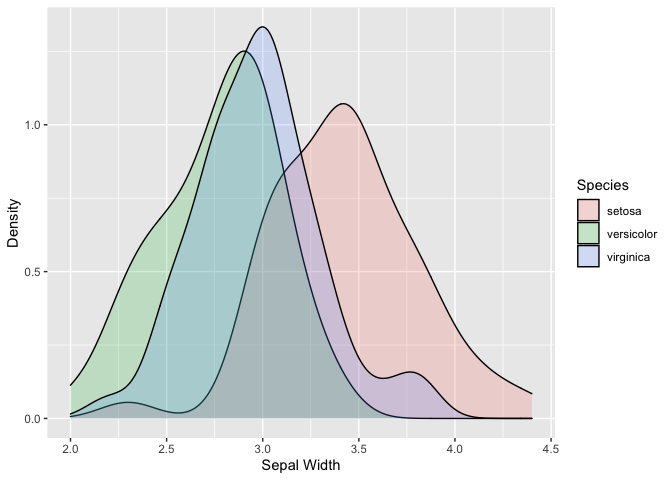
(\#fig:Figure2)My amazing figure

Using `bookdown::html_document2`, I can reference Figure \@ref(fig:FigureExample) and \@ref(fig:Figure2). It is important to **label your figure chunks without spaces or special characters** to make this work.

Using bookdown::html_document2, I can reference Figure \@ref(fig:FigureExample) and \@ref(fig:Figure2). It is important to label your figure chunks without spaces or special characters to make this work.

While working with LaTeX, it is good to manually introduce the figure in an environment to gain control over the plot settings. Considering the case of \@ref(fig:Figure2), let’s see an example:

{=latex}
\begin{figure}[H]
\caption{Your Caption \label{fig:fig:label}}

{r Figure2_Latex, echo=FALSE}
# The code of this plot was extracted from https://www.publichealth.columbia.edu/sites/default/files/media/fdawg_ggplot2.html
library(ggplot2)
density2 <- ggplot(data=iris, aes(x=Sepal.Width, fill=Species))
density2 + geom_density(stat="density", alpha=I(0.2)) +
  xlab("Sepal Width") +  ylab("Density") + ggtitle("Histogram & Density Curve of Sepal Width")

{=latex}
\begin{minipage}{\textwidth}
\footnotesize \textbf{Notes}: Notes... \par
\end{minipage}
\end{figure}

Equations

`R Markdown` comes with LaTeX incorporated. You can write environments, equations and use most of the LaTeX capabilities inside your notebooks. Let's see some examples:

$$E = mc^2$$

R Markdown comes with LaTeX incorporated. You can write environments, equations and use most of the LaTeX capabilities inside your notebooks. Let’s see some examples:

\[E = mc^2\]

You also can number equations using equation environment together with a label.

\begin{equation}
\hat{\beta} = (X'X)^{-1}X'Y (\#eq:eq1)
\end{equation} 
 
The model \@ref(eq:eq1) are the estimated coefficients by OLS.

You also can include tikz graphs inside your R Markdown documents if you are compiling a PDF. This functionality will not work in HTML or other outputs. Check this SO question to see more information.

\begin{tikzpicture}
\begin{axis}[xmax=9,ymax=9, samples=50]
  \addplot[blue, ultra thick] (x,x*x);
  \addplot[red,  ultra thick] (x*x,x);
\end{axis}
\end{tikzpicture}

# Code from https://stackoverflow.com/questions/27880563/tikz-in-r-markdown

Configuring the document with YAML

Another thing that I love from R Markdown is that the global configuration of the document is with YAML. According to Wikipedia, ““YAML (a recursive acronym for “YAML Ain’t Markup Language”) is a human-readable data serialization language. It is commonly used for configuration files and in applications where data is being stored or transmitted”.

This way of configuring a document is far easier than LaTeX preambles (not recommended for humans), mainly because YAML is readable. For example, the header of this R Markdown looks like this:

title: "All you need is `R Markdown`!"
output: 
  bookdown::html_document2:
    keep_md: True
    toc: no

For example, if I would like to add a Table of Contents and not keep the Markdown file as the output of the R Markdown, the header will look like this:

title: "All you need is `R Markdown`!"
output: 
  bookdown::html_document2:
    keep_md: False
    toc: yes

In addition, this is the place to include a bibliography for your document. R Markdown supports json, bibtex, and many other formats!

title: "All you need is `R Markdown`!"
output: 
  bookdown::html_document2:
    keep_md: False
    toc: yes
bibliography: bibliography.extension

For more configurations, I suggest this guide.

My manuscript template.

Another cool stuff about R Markdown is that you can use your own LaTex template to configure your PDF document. By default, R Markdown has many templates to compile a document in PDF using LaTeX. Inspired by Aidan Milliff’s template, I created my own template for manuscripts. The header of my R Markdown document looks like:

---
output: 
  pdf_document:
    citation_package: natbib
    latex_engine: pdflatex
    template: rm_tex_ms_template.tex
title: "Title"
subtitle: "Subtitle"
thanks: "Acknowledgements"
date: # Today, unless specified. In smaller font if specified to allow for version numbering
author:
- name: Author 1
  affiliation: Affiliation 1
  mail: author1@yourmail.com
- name: Author 2
  affiliation: Affiliation 2
  mail: author1@yourmail.com
- name: Author 3
  affiliation: Affiliation 3
  mail: author1@yourmail.com
- name: Author 4
  affiliation: Affiliation 4
  mail: author1@yourmail.com
abstract: 
  text: "In here you can write the abstract of your amazing academic paper. Blah Blah Blah my paper is awesome, don't reject it."
  size: "'footnotesize'"
keywords: Key1, Key2, Key3
jelcodes: JEL1, JEL2, JEL3
# Document Class Options
dc_options:
  fontsize: 12pt
# Fontfamily options Class Options
fontfamily: mathpazo
toc: false
geometry: margin= 1in
#spacing: onehalf
bibliography: 
biblio-style: apsr
citecolor:
urlcolor:
linkcolor: blue
anonymous: false # quickly sanitizes manuscript for blind review if 'true'
---

With this header, I configure my LaTeX documents. It is important to have the template in the same directory as the .Rmd when using this same header. If you want to move the template to another directory, you must specify the route in template: path/to/the/rm_tex_ms_template.tex. You can find the template and the compiled PDF in my GitHub!

Final Thoughts

In these last months, R Markdown has been a handy tool to perform statistical analysis and present my progress to my teammates without. R Markdown has helped me concentrate my time on the data analysis rather than moving outputs from my codes to external documents. In this post, I share most of my tips and tricks that I use daily, and I hope this will help you work smarter in the future!

References and Further reading

***********************